Part 1 – How much storage space and processing time will be required?
Are you a researcher who wants to quantify human behaviour, physiology or environmental conditions? Have you decided to utilise sensor data? Good idea! Sensor data is generally continuously monitored and objective, so it provides fine-grained, reliable data.
This can be preferable to qualitative ‘self-reporting’ methods or AI methods, which might be time-consuming to collect, more subjective and/or less reliable.
There are a few things that you need to think about though, before you embark on your data collection and storage, so keep reading and we’ll guide you through the two main questions that we are often asked:
- How much storage space will I need?
- How long will it take to process?
To illustrate the answers to these questions, we simulated a typical data cleaning and pre-processing pipeline, run on dummy data, on a typical UoM issue laptop.
How much storage space will my sensor data require?
Most research projects will be working with raw sensor data straight from the devices. Raw sensor data is not cleaned or pre-processed in any way. This gives users (e.g. researchers) the flexibility to make their own decisions about what data to delete and how to process any anomalies, but it can also mean that you receive/download a lot more data than you require. Even if data download facilities have excellent filtering mechanisms, you might still find yourself downloading data that you won’t eventually need.
Unprocessed sensor data is timeseries data, and it is often very large. The size can increase (sometimes exponentially) with the following factors:
- How many sensors are being used in your study? There are many different sensors, e.g. human-wearable devices, and air quality sensor. If human-wearable devices are being used, then the number of sensors is the number of participants in the study.
- How many fields are being recorded. Each sensor can record multiple fields, for example temperature, pH, CO2, NO2, heart-rate and step-count. The raw data recording process often collects the data in separate files, one for each field. Note also, that when you collect raw sensor data there are likely to be ’extra’ fields that you don’t need, (or that you’re not yet sure if you will need them) and that you still need to store prior to cleaning your data.
- The length of time (e.g. how many days) you are recording data for.
- Sample frequency: How often the sensor collects the data. For example, is the data collected for every day, hour, minute, second, or more frequently?
To give an idea of data sizes, we can make some rough calculations of how much data an example project would need to store, measured in datapoints. We define a datapoint as a single measurement value for a single sensor at a single point of time. You might think of it as a single cell in a spreadsheet made up of one row per time-stamped data collection instance and a column for each measurement.
Our dummy datasets
We have generated dummy datasets with the following characteristics:
- 50 sensor devices (e.g. 50 participants who each wear a smart-watch sensing device)
- 4 measurements from each sensor device.
- for 6 months (182 days)
- We generate 3 datasets: collecting a measurement for every hour, minute and second respectively.
For the minute-interval dataset, the number of datapoints (including the sensor-ID and timestamp fields) is:
50 (sensors/participants) x 6 (4 measurements + sensor ID and timestamp) x 182 days x 1140 (60 minutes x 24 hours)
= 73,164,000 datapoints = 10,374,000 rows with 6 columns = approx. 0.86 GB data.
If we increase the time-granularity to every second, then we multiply the above by 60 and you get approximately 50 GB of data.
Note that the above calculations exclude any unrequested extra fields that you may also need to download and store before removing them. In addition, many sensor datasets contain duplicate rows that need to be removed during cleaning.
What will happen if I process sensor data on my laptop?
To answer this question, Ann Gledson, one of our Research Software Engineers (RSE) has generated the dummy sensor data described above, for hour, minute and second intervals. She has written a Python script, utilising the Pandas library (a well-known, fast, powerful Python data processing module) that performs data wrangling. Research Platforms Engineer (RPE) Abhijit Ghosh has set up a test environment on the CSF that mimics a typical UoM-issued laptop from the standard ITS catalogue. For comparison, further test environments have been added with more CPU cores and memory.
The data wrangling tasks used in our experiment
The Python script performs some typical data cleaning/processing tasks:
- Deduplicating records with identical sensor IDs and date-time values.
(Our dummy dataset contains 2% duplicates) - Resample the time-series to be 1 record/row per day
- Group by sensor ID (resulting in one record per sensor / day)
- Calculate the count, mean, sum and standard deviation (std) for each sensor/measurement/day.
- Save the output file to a new CSV file, having columns for day, sensor, and count, mean, sum and std for each measurement.
List of assumptions
Every research project is different, but for these calculations, we need to start somewhere, so here is our list of assumptions. We feel that these represent common data wrangling scenarios:
- No geo-location data is required. Sensors that are moving (wearable devices) often have geo-location information, and if you need to use that, it will take up extra processing time.
- The data measurements are stored in columns within the same raw data (csv) file
rather than in separate files for each measurement. If stored separately, these would need to be joined, which would require more processing time. - Each data file is in CSV format, and there is 1 file per sensor ID (e.g. one file per participant, who is wearing a sensing device such as a sports watch).
- Data processing is done on a machine with 16GB of RAM. This is the typical current RAM (random access memory - short-term memory for storing data being used by calculations) for standard work laptops.
- 1 core processor is being used. Typical laptops will have 2-4 CPU cores, but these are to allow multi-tasking of typical laptop functions of running applications side-by-side, rather than running computationally intensive (i.e. data processing) applications.
Comparison with using Research IT CSF3
For comparison, we also show results for when using up to 32 CPU cores, but this would not be found on a standard laptop. A single serial job in CSF3 provides a single 2.8GHz CPU core and 8GB of RAM which is roughly equivalent to running the script on a laptop having a CPU with a similar clock speed and 16GB RAM, (a part of which, as mentioned above, is already used up by the Operating System and other software/processes running on the laptop). The 2, 4, 8, 16 and 32 core tests were run on the CSF3 on the same or similar CPU cores. CSF3 can provide 6GB per core to 128GB per core RAM and can also provide up to 4TB of dedicated RAM for your jobs. This is simply not possible on a laptop.
Two ways to run the data wrangling
As we are assuming that we have 1 file per Sensor ID, when only using a single CPU core, there are two ways that we have processed this data:
- Method A: When running on a single CPU core, we could join all these files into one (much larger) dataset and then run the data wrangling procedures on that. This is a memory-hungry approach, but it may be required if you need to run any aggregation functions (e.g. sum, mean, standard deviation, max) on the entire dataset.
- Method B: We could keep the files separate for the data-wrangling tasks and then join the resulting (much smaller) files at the end, taking up much less memory (RAM). (This method is used for those tests using more than one CPU core.)
Results for Method A
Processing times for these two different methods, using between 1 and 32 cores, are shown below.
The 2, 4, 8, 16 and 32 core tests were ran on CSF3 on same/similar CPU cores. CSF3 can provide 6GB per core to 128GB per core RAM and can also provide up to 4TB of dedicated RAM for your jobs. This is simply not possible on a laptop.
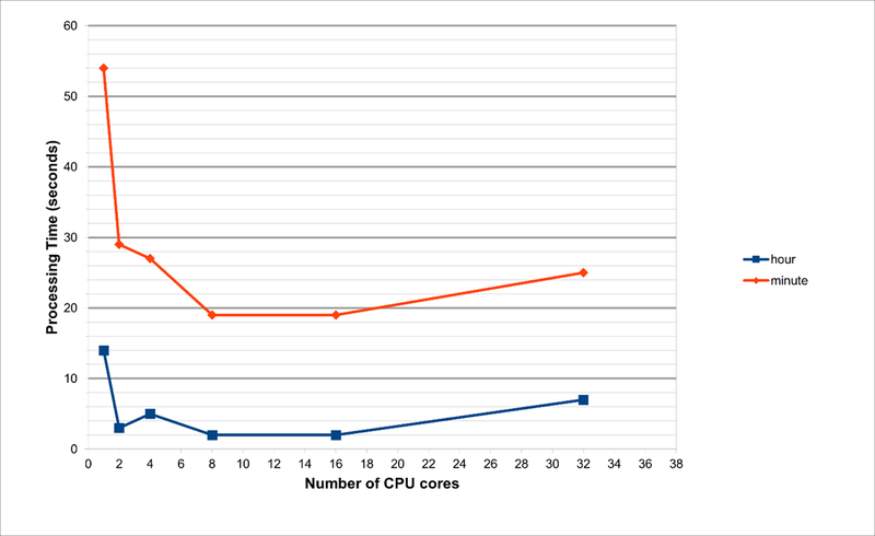
Note that for the second-interval data, when running on 1 processor, the time taken is around 1700 seconds, or 28 minutes. Furthermore, the RAM requirements are 132GB and 135GB when using 1 or 2 processors, respectively. Due to these huge memory requirements, these jobs are impossible to run on any normal laptop (or even Workstations, unless there is sufficient RAM). This is because we are joining all the data files into a single dataset, and this needs to be held in memory while the wrangling functions are run.
As per our tests and as evident from the charts, the optimum number of CPU cores to run the code is 8. This is not possible on a laptop with 4-cores. With hyperthreading turned on, one can run an 8-core job on a processor that supports hyperthreading with just 4-cores, but the performance will be suboptimal. Also, the laptop will begin to heat up and freeze with such usage.
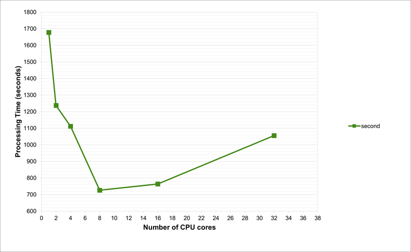
Results for Method B
(Second-interval data only)
Method B would be the preferred way of running the data-wrangling, if no aggregate functions are needed to be run on the entire dataset. This method was found to be more efficient, using only 3GB of RAM, but the processing time on a typical laptop, with a single processor is still around 22 minutes.
Summary
To summarise, even with a very conservative estimate, using only 50 sensors, each recording 4 measurements, every second, over 6 months, the downloaded dataset will take up around 50GB of storage. Running basic data-wrangling processes to clean up this data is likely to cause problems if using a laptop, as we can generally only use 1 or 2 processor cores and the maximum RAM is around 16GB (sometimes lower). The above jobs will take between 22 and 28 minutes to run, and there is a good chance that your laptop may slow down or even freeze whilst running.
If you think that your sensor dataset is likely to take up a lot of storage and processing power, rest assured that Research IT has easy-to-use, shared resources that you can use. In Part 2, we will look at these other options available to UoM researchers for storing and processing sensor data, such as our Research Data Storage (RDS) and Computational Shared Facility (CSF) and we will provide some easy-to-follow guidelines on how to use them.